Kaggle —”Getting Started” - Digit Recognizer

https://unsplash.com/@ikukevk

A series of short blog on how to solve the basic initial tasks of Kaggle.

All of the tasks have achieved best of their results. Not to miss, I have had taken help from other notebooks in Kaggle when I was not able to reach the goal.

So here I’m trying to explain a bit in detail all the “Getting Started Tasks” in Kaggle. To again repeat myself the basic tasks helps to acquiring knowledge on Computer Vision, Data Science and NLP.

So when it comes to Computer Vision based tasks we are exploring the Digit Recognizer from MNIST datasets. Below one can find the flow of the task, followed by short descriptions and intermittent code for complete understanding.

The flow of the task to solve Digit Recognizer can be as given below

• Introduction
• Data Exploration
• CNN Model
• Model Verification

Each of the section again has subsections which can be seen in later stages. The result however is shown in brief. The accuracy of 98% was achieved over this architecture and method.

Introduction

In this practice, 6 layers Sequential Convolutional Neural Network is trained using MNIST dataset for digit recognizer. The model is built using Keras code, so this code looks more intuitive. Unlike statistical learning, feature extraction based model training does not need much of the pre-processing work. But one should have an idea of covering all the required data in the form of images, augment the data and train the model to perfection. This is exactly where core knowledge comes to picture.

Load all the required libraries:

Load the libraries

Data Exploration

• Load Data: Load the data from CSV, copy the targets to standard variable and visualize the plot for inequality in the classes if any.

Code to load data and visualize

Histogram of MNIST dataset

There is nothing much to worry about the inequality of the classes. Since the histogram shows no partiality with the classes.

• Handle missing and null values: Luckily, here we are dealing with the image data. If it was any of the other data then various categories in data like categorical, numeric and binary would come into picture. But nevertheless, to be on safer side lets examine if we have any missing data or null values. The below code helps in getting the confirmation about it.

Code to check for missing values

Check for missing values

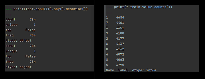
There are no missing values in this MNIST data.

• Normalize, reshape: Since the ConvNets converge faster when the data ranges between [0..1] than on [0..255], let’s normalize the data. Also, technically grayscale normalization reduces the effect of illumination’s differences. Normalize is done by dividing by the max of the pixel data. Along with this the reshape of data is done. Since the image are of dimension 28*28*1. Below is code snippet.

Code to Normalize and Reshape

• Label encoding: One hot vector is formed which is actually utilized during the loss function. Since our values ranges between [0..1] this one hot vector eases the calculation task.

Encode into one hot vector

• Splitting the data [Train, Validation]: Usual trend of any machine learning task to split the data. Here, i have allocated the 10% to validation for evaluation of the model and 90% of the data to training. Random split is done to consider avoid unequal distribution of the data.

Code to split the data

CNN

As i mentioned before Keras code looks more intuitive, one layer at a time is added starting from the input. It is basically a sequential API. Here I have 5 layers, the first 2 layers consists of 32 filters followed by next 3 layers of 64 filters. These filters are learnable filters. The input layer is succeeded by the convolution layer. Filters are used in this layer, which are also called kernel. The filter is an array or matrix of numbers, these numbers are called weights. The depth of the filters are expected to be same as the input layer depth. These CNN filters helps in extracting the features.

The next important layer is Max Pooling. Most commonly called down-sampling layer is the pooling layer. There are many variations
available to use in this layer. Max pooling is one of the common logic used. The pooling layer usually considers filter and stride of same length. It then outputs the maximum number in every sub-region of the input area, that the filter overlaps with

With the combination of convolution and pooling layers local and global features are extracted and this helps the model to train the model to perfection.

Regularization method such as dropout is used in here. This is to avoid over-fitting and to improve the generalization of the neural network. The activation function used here is ReLU which helps in adding the non-linearity to the network. Softmax function is used as an activation function to squeeze the neurons output between the value of 0 and 1 to give the probability of each class.

Code for CNN model

Once all the layers are set up optimization algorithm and loss function is set-up. The loss function gives the error rate between the predicted and observed outputs. Here, categorical entropy loss function is used. The optimizer function helps in iteratively improving the weights, bias and filter kernel values. In turn these will decrease the error rate. Here RMSprop is adopted. Accuracy is used to evaluate the performance of the model.

Code for Optimizer

In order to minimize the error at much faster rate and to find the global minimum of the loss function, a parameter to improve the learning rate needs to be added.
This basically reduces the learning rate when a metric has stopped improving. From this models often benefits when the learning rate factor is reduced by 2–10. The argument patience monitors when to decrease the learning rate. If there is no improvement for patience number of epochs, the learning rate is reduced. Here, the learning rate is reduced by 40%

Code for monitoring LR

Data Augmentation is a technique to avoid over-fitting. This technique also improves the performance of the model by augmenting the data we already have. It also generalizes and artificially expands the size of a training dataset by creating modified versions of images in the dataset. Few of the techniques that are available in data augmentation are flipping (vertical or horizontal), rotation (rotates by specific degree), shearing (shifts one part of the image like a parallelogram), cropping (random crop at different positions in different propositions), Zoom in and out, brightness and contrast.
With these augmentation technique there is definitely a room to increase the data and generalize the model. Here, in this model random rotation by 20%, random zoom by 20%, random shift horizontal by 20% and random shift vertical by 20% are employed. Without data augmentation the accuracy of the model would be definitely less.

Code for Data Augmentation

Verification

The results can be verified by predicting using the below code.

Code to predict results